[译] [论文] BBR:基于拥塞(而非丢包)的拥塞控制(ACM, 2017)
译者序
本文翻译自 Google 2017 的论文:
Cardwell N, Cheng Y, Gunn CS, Yeganeh SH, Jacobson V. BBR: congestion-based congestion control. Communications of the ACM. 2017 Jan 23;60(2):58-66.
论文副标题:Measuring Bottleneck Bandwidth and Round-trip propagation time(测量瓶颈带宽和往返传输时间)。
BBR 之前,主流的 TCP 拥塞控制算法都是基于丢包(loss-based)设计的, 这一假设最早可追溯到上世纪八九十年代,那时的链路带宽和内存容量分别以 Mbps 和 KB 计,链路质量(以今天的标准来说)也很差。
三十年多后,这两个物理容量都已经增长了至少六个数量级,链路质量也不可同日而语。特别地,在现代基础设施中, 丢包和延迟不一定表示网络发生了拥塞,因此原来的假设已经不再成立。 Google 的网络团队从这一根本问题出发,(在前人工作的基础上) 设计并实现了一个基于拥塞本身而非基于丢包或延迟的拥塞控制新算法,缩写为 BBR。
简单来说,BBR 通过应答包(ACK)中的 RTT 信息和已发送字节数来计算 真实传输速率(delivery rate),然后根据后者来调节客户端接下来的 发送速率(sending rate),通过保持合理的 inflight 数据量来使 传输带宽最大、传输延迟最低。另外,它完全运行在发送端,无需协议、 接收端或网络的改动,因此落地相对容易。
Google 的全球广域网(B4)在 2016 年就已经将全部 TCP 流量从 CUBIC 切换到 BBR, 吞吐提升了 2~25 倍;在做了一些配置调优之后,甚至进一步提升到了 133 倍(文中有详细介绍)。
Linux 实现:
include/uapi/linux/inet_diag.hnet/ipv4/tcp_bbr.c
翻译时适当加入了一些小标题,另外插入了一些内核代码片段(基于内核 5.10),以更方便理解。
由于译者水平有限,本文不免存在遗漏或错误之处。如有疑问,请查阅原文。
以下是译文。
- 译者序
- 1 拥塞和瓶颈(Congestion and Bottlenecks)
- 2 瓶颈的数学表示(Characterizing the Bottleneck)
- 3 使数据流(Packet Flow)与传输路径(Delivery Path)相匹配
- 4 BBR Flow 行为
- 5 部署经验
- 6 问题讨论
- 7 总结
- 致谢
- 附录:详细描述
- References
从各方面来说,今天的互联网传输数据的速度都不甚理想:
- 大部分移动用户都在忍受数秒乃至数分钟的延迟;
- 机场和大会场馆的共享 WIFI 信号一般都很差;
- 物理和气候学家需要与全球合作者交换 PB 级的数据,最后却发现精心设计的 Gbps 基础设施在跨大洲通信时带宽经常只能达到 Mbps6。
这些问题是由 TCP 的设计导致的 —— 20 世纪 80 年代设计 TCP 拥塞控制(congestion control) 时,认为丢包是发生了“拥塞”13。 在当时的技术条件下我们可以这样认为,但它并非第一原则 (technology limitations, not first principles)。随着网卡从 Mbps 到 Gbps、 内存从 KB 到 GB,丢包和拥塞之间的关系也变得愈发微弱。
今天,TCP 那些基于丢包的拥塞控制(loss-based congestion control) —— 即使是目前其中最好的 CUBIC11 —— 是导致这些问题的主要原因。
- 链路瓶颈处的 buffer 很大时,这类算法会持续占满整个缓冲区,导致 bufferbloat;
- 链路瓶颈处的 buffer 很小时,这类算法又会误将丢包当作拥塞的信号,导致吞吐很低。
解决这些问题需要一种全新的方式,而这首先需要对以下两点有深入理解:
- 拥塞会发生哪里(where)
- 拥塞是如何发生的(how)
1 拥塞和瓶颈(Congestion and Bottlenecks)
1.1 两个物理特性:传输时延(RTprop)和瓶颈带宽(BtlBw)
对于一个(全双工)TCP 连接,在任意时刻,它在每个方向都有且只有一段最慢的链路 (exactly one slowest link)或称瓶颈(bottleneck)。这一点很重要,因为:
-
瓶颈决定了连接的最大数据传输速率。这是不可压缩流(incompressible flow)的一个常规特性。
例如,考虑交通高峰期的一个六车道高速公路,一起交通事故使其中一段变成了单车道, 那么这整条高速公路的吞吐就不会超过那条唯一还在正常通车的车道的吞吐。
-
瓶颈也是持久队列(persistent queues)形成的地方。
对于一条链路,只有当它的离开速率(departure rate)大于到达速率(arrival rate)时,这个队列才会开始收缩。对于一条有多段链路、运行在最大传输速率的连 接(connection),除瓶颈点之外的地方都有更大的离开速率,因此队列会朝着瓶颈 移动(migrate to the bottleneck)。
不管一条连接会经过多少条链路,以及每条链路的速度是多少,从 TCP 的角度来看, 任何一条复杂路径的行为,与 RTT(round-trip time)及瓶颈速率相同的单条链路的行为是一样的。 换句话说,以下两个物理特性决定了传输的性能:
RTprop(round-trip propagation time):往返传输时间BtlBw(bottleneck bandwidth):瓶颈带宽
如果网络路径是一条物理管道,那 RTprop 就是管道的长度,而 BtlBw 则是管道最窄处的直径。
1.2 传输时延/瓶颈带宽与 inflight 数据量的关系
图 1 展示了 inflight 数据量(已发送但还未被确认的数据量)不断增大时, RTT 和传输速率(delivery rate)的变化情况:
直观上,这张图想解释的是:随着正在传输中的数据的不断增多,传输延迟和传输速率将如何变化。 难点在于二者并没有简单的关系可以表示。不仅如此,后文还将看到二者甚至不可同 时测量 —— 就像量子力学中位置和动量不可同时测量。 译注。
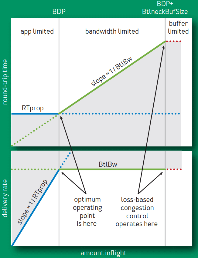
Fig 1. Delivery rate and RTT vs. inflight data
- 蓝线展示 RTprop 限制,
- 绿线展示 BtlBw 限制,
- 红线是瓶颈缓冲区(bottleneck buffer)
横轴表示 inflight 数据量,关键的点有三个,依次为 0 -> BDP -> BDP+BtlneckBuffSize,
后两个点做垂线,将整个空间分为了三个部分:
(0, BDP):这个区间内,应用(客户端)发送的数据并未占满瓶颈带宽(容量),因此称为 应用受限(app limited)区域;(BDP, BDP+BtlneckBuffSize):这个区间内,已经达到链路瓶颈容量,但还未超过 瓶颈容量+缓冲区容量,此时应用能发送的数据量主要受带宽限制, 因此称为带宽受限(bandwidth limited)区域;(BDP+BtlneckBuffSize, infinity):这个区间内,实际发送速率已经超过瓶颈容量+缓冲区容量 ,多出来的数据会被丢弃,缓冲区大小决定了丢包多少,因此称为缓冲区受限(buffer limited)区域。
以上三者,也可以更直白地称为应用不足、带宽不足、缓冲区不足区域。 译注。
1.3 以上关系的进一步解释
我们来更具体地看一下传输时延(RTprop)和瓶颈带宽(BtlBw)与与 inflight 数据量呈现以上关系:
-
inflight 数据量在
0 -> BDP区间内时,发送的数据还未达到瓶颈容量,此时,- 往返时间不变:对应上半部分图,因为此时还未达到瓶颈带宽,链路不会随数据量增加而带来额外延迟;
- 传输速率线性增大:对应下半部分图;
因此,这个阶段的行为由 RTprop 决定。
-
inflight 数据量刚好等于
BDP时,- 两条限制线相交的点称为 BDP 点,这也是 BDP(bandwidth-delay product,带宽-延迟乘积)这个名称的由来;
- 此时可以算出:
inflight = BtlBw × RTprop;
-
inflight 大于
BDP之后,管道就满了(超过瓶颈带宽)- 超过瓶颈带宽的数据就会形成一个队列(queue),堆积在链路瓶颈处,然后
- RTT 将随着 inflight 数据的增加而线性增加,如上半部分图所示。
-
inflight 继续增大,超过
BDP+BtlneckBuffSize之后,即超过链路瓶颈所支持的最大缓冲区之后,就开始丢包。
灰色区域是不可达的,因为它违反了至少其中一个限制。限制条件的不同导致了三个可行区域 (app-limited, bandwidth-limited, and buffer-limited)各自有不同的行为。
1.4 拥塞和拥塞控制的直观含义
再次给出图 1,
Fig 1. Delivery rate and RTT vs. inflight data
直观上来说, 拥塞(congestion)就是 inflight 数据量持续向右侧偏离 BDP 线的行为, 而拥塞控制(congestion control)就是各种在平均程度上控制这种偏离程度的方案或算法。
1.5 基于丢包的拥塞控制工作机制
基于丢包的拥塞控制工作在 bandwidth-limited 区域的右侧,依靠:
- 很高的延迟,以及
- 频繁的丢包
将连接的传输速率维持在全速瓶颈带宽(full bottleneck bandwidth)。
- 在内存很贵的年代,瓶颈链路的缓冲区只比 BDP 略大,这使得 基于丢包的拥塞控制导致的额外延迟很小;
- 随着内存越来越便宜,缓冲区已经比 ISP 链路的 BDP 要大上几个数量级了, 其结果是,bufferbloat 导致的 RTT 达到了秒级,而不再是毫秒级9。
1.6 更好的工作机制及存在的挑战
Bandwidth-limited 区域的左侧边界是比右侧更好的一个拥塞控制点。
- 1979 年,Leonard Kleinrock16 证明了这个点是最优的, 能最大化传输速率、最小化延迟和丢包,不管是对于单个连接还是整个网络8。
- 不幸的是,大约在同一时间,Jeffrey M. Jaffe14 证明了 不存在能收敛到这个点的分布式算法。这个结果使得研究方向从寻找一个能达到 Kleinrock 最佳工作点(operating point)的分布式算法,转向了对不同拥塞控制方式的研究。
在 Google,我们团队每天都会花数小时来分析从世界各地收集上来的 TCP 包头, 探究各种异常和反常现象背后的意义。
- 第一步通常是寻找基本的路径特性 RTprop 和 BtlBw。
- 能从跟踪信息中拿到这些数据这一事实,说明 Jaffe 的结论可能并没有看上去那么悲观。 Jaffe 的结果在本质上具有测量模糊性(fundamental measurement ambiguities),例 如,测量到的 RTT 增加是由于路径长度变化导致的,还是瓶颈带宽变小导致的,还是另 一个连接的流量积压、延迟增加导致的。
- 虽然无法让任何单个测量参数变得很精确,但一个连接随着时间变化的行为 还是能清晰地反映出某些东西,也预示着用于解决这种模糊性的测量策略是可行的。
1.7 BBR:基于对两个参数(RTprop、BtlBw)的测量实现拥塞控制
组合这些测量指标(measurements),再引入一个健壮的伺服系统 (基于控制系统领域的近期进展) 12,我们便得到一个能针对对真实拥塞 —— 而非丢包或延迟 —— 做出反应的 分布式拥塞控制协议,能以很大概率收敛到 Kleinrock 的最优工作点。
我们的三年努力也正是从这里开始:试图基于对如下刻画一条路径的两个参数的测量, 来实现一种拥塞控制机制,
- 瓶颈带宽(Bottleneck Bandwidth)
- 往返传输时间(Round-trip propagation time)
2 瓶颈的数学表示(Characterizing the Bottleneck)
2.1 最小化缓冲区积压(或最高吞吐+最低延迟)需满足的条件
当一个连接满足以下两个条件时,它将运行在最高吞吐和最低延迟状态:
-
速率平衡(rate balance):瓶颈链路的数据包到达速率刚好等于瓶颈带宽
BtlBw,这个条件保证了链路瓶颈已达到 100% 利用率。
-
管道填满(full pipe):传输中的总数据(inflight)等于 BDP(
= BtlBw × RTprop)。这个条件保证了有恰好足够的数据,既不会产生瓶颈饥饿(bottleneck starvation), 又不会产生管道溢出(overfill the pipe)。
需要注意,
-
仅凭 rate balance 一个条件并不能确保没有积压。
例如,某个连接在一个 BDP=5 的链路上,开始时它发送了 10 个包组成的 Initial Window,之后就一直稳定运行在瓶颈速率上。那么,在这个链路此后的行为就是:
- 稳定运行在瓶颈速率上
- 稳定有 5 个包的积压(排队)
-
类似地,仅凭 full pipe 一个条件也无法确保没有积压。
例如,如果某个连接以
BDP/2的突发方式发送一个 BDP 的数据, 那仍然能达到瓶颈利用率,但却会产生平均 BDP/4 的瓶颈积压。
在链路瓶颈以及整条路径上最小化积压的唯一方式是同时满足以上两个条件。
2.2 无偏估计(unbiased estimator)
下文会提到“无偏估计”这个统计学术语,这里先科普下:
In statistics, the bias (or bias function) of an estimator is the difference between this estimator’s expected value and the true value of the parameter being estimated. An estimator or decision rule with zero bias is called unbiased.
Wikipedia: Bias of an estimator
译注。
2.3 传输时延(RTProp)的表示与估计
BtlBw 和 RTprop 在一个连接的生命周期中是不断变化的,因此必须持续对它们做出估计(estimation)。
TCP 目前跟踪了 RTT(从发送一段数据到这段数据被确认接收的时间) ,因为检测是否有丢包要用到这个参数。在任意时刻 t,

其中
- 𝛈 ≥ 0 表示路径上因为积压、接收方延迟应答策略、应答聚合等因素而引入的“噪声”;
- RTprop 是往返传输时延。
前面已经提到,RTprop 是路径(connection’s path)的一个物理特性,只有当路径发
生变化时它才会变化。由于路径变化的时间尺度远大于 RTProp,因此在时刻 T,一个无偏、高效估计是:

例如,在时间窗口 WR 内的移动最小值(running min),其中典型情况下, WR 的持续时间是几十秒到几分钟。
这里直观上的解释是:一段时间内的最小 RTT(可测量),就是 这条路径(在一段时间内)的往返传输延迟。 译注。
2.4 瓶颈带宽(BtlBw)的表示与估计
不同于 RTT,TCP 规范中并没有要求跟踪 bottleneck bandwidth,但可以通过 跟踪传输速率(delivery rate)来得到一个对瓶颈带宽的不错估计。
当应答包(ACK)到达发送端时,其中除了包含 RTT 信息,还包含包离开时的 inflight data 传输情况。已传输的数据量除以传输时间,就是发送和应答之间的平均传输速率:
deliveryRate = Δdelivered/Δt
- 这个速率一定
<= bottleneck rate; - 到达数据量 Δdelivered 已经知道了,因此接下来需要确定的是 Δt,而 Δt ≥ true arrival interval;
- 因此,
deliveryRate <= the true delivery rate,也就是估计出的传输速率,不会超过真实瓶颈带宽,后者是前者的上限。
因此,传输速率在一段时间窗口内的最大值(windowed-max),是 BtlBw 的一个高效、 无偏估计:

其中时间窗口 WB 典型情况下是 6~10 个 RTT。
这里直观上的解释是:一段时间内的链路最大传输带宽(可测量),就是这条链路的瓶颈带宽。 译注。
2.5 BBR 测量机制
TCP 记录了每个包的离开时间,再加上已传输的数据量,当每个 ACK 包到达发送端时,将产生:
- 一个 RTT 值
- 传输速率的一次测量值(a delivery rate measurement)
过滤器可以将这两个测量到的值转换成对 RTprop 和 BtlBw 的估计。
注意,这两个变量是完全独立的:
- 在瓶颈带宽不变的情况下,RTprop 仍可能发生变化(例如,路由变了);
- 路径(path)不变的情况下(因此 RTprop 也不变),BtlBw 也可能发生变化(例如,某条无线链路速率变了)
这种无关性也解释了为什么需要同时知道这两个限制条件,才能确定传输路径的发送行为。
2.6 不确定性原理
由于 RTprop 只对 BDP 的左侧可见,BtlBw 只对右侧可见,因此它们服从不确定性原理( uncertainty principle):当测量其中一个时,另一个将不可测量。
直观上的解释是:管道整个长度被填满 —— 或称溢出(overfilled)—— 时才能达到它的 最大容量,而溢出之后会(在缓冲区中)创建一个队列(queue),后者作为管道的 延伸又反过来模糊了管道的长度。
例如,
- 发送请求/接收响应的的应用:可能永远无法发送足够多的数据来填满管道,因此它 只能测量到传输延迟,而无法测量到 BtlBw。
- 持续几小时的大批量数据传输:可能整个生命周期都位于图中的带宽受限区域,因此它 自始至终只有一个 RTprop 样本,也就是第一个包的 RTT(其他包 的 RTT 对这种场景来说是无效样本)。
这种内在的不确定性意味着,除了依靠测量值来估计(恢复)出两个路径变量之外, 必须有状态来跟踪:
- 从当前的工作位置可以学到什么(what can be learned at the current operating point)
- 当信息失效时,如何找到下一个可以继续学习的工作位置(how to get to an operating point where it can be relearned)
这里说的“工作位置”,是指图 1 中的 RTProp 和 BtlBw 不同组合产生的位置。
3 使数据流(Packet Flow)与传输路径(Delivery Path)相匹配
BBR 的核心算法分为两部分:
- 当收到一个 ACK 时,应该做什么操作;
- 当发送一段数据时,应该做什么操作。
3.1 BBR 收到应答包(ACK)时的逻辑
每个 ACK 都为我们提供了 RTT 和平均传输速率 的一次测量,二者又将分别更新对 RTprop 和 BtlBw 的估计。
具体来说,收到一个 ACK 时,BBR 将执行以下逻辑:
function onAck(packet)
  rtt = now - packet.sendtime                      // 收包时间 减去 包中记录的发包时间
  update_min_filter(RTpropFilter, rtt)             // 根据 2.2 中的方程,更新对 RTT 的估计

  delivered      += packet.size
  delivered_time =  now
  delivery_rate  =  (delivered - packet.delivered) / (delivered_time - packet.delivered_time)

  if (delivery_rate > BtlBwFilter.current_max      // 实际传输速率已经大于当前估计的瓶颈带宽,或
     || !packet.app_limited)                       // 不是应用受限(应用受限的样本对估计 BtlBw 无意义)
     update_max_filter(BtlBwFilter, delivery_rate) // 根据 2.3 中的方程,更新对 BtlBw 的估计

  if (app_limited_until > 0)                       // 达到瓶颈带宽前,仍然可发送的字节数
     app_limited_until = app_limited_until - packet.size
几点说明:
- 每个包都会更新对 RTProp 的估计,但只有部分包会更新对 BtlBw 的估计;
-
应用受限的包
- 对于一个包,当应用(application)全速发送它而仍然没有占满瓶颈带宽时,
BBR 会这个包标记为
app_limited(见下面的send()伪代码), 即packet.app_limited = true。 - 这将决定哪些样本会用来更新对带宽的估计。
- 对于一个包,当应用(application)全速发送它而仍然没有占满瓶颈带宽时,
BBR 会这个包标记为
-
瓶颈带宽 BtlBw 是传输速率的一个硬性上限,因此
- 如果测量到当前的传输速率 > 当前对 BtlBw 估计,
必定意味着这个估计太低了,不管样本是不是 app-limited;对应到上面的代码,就是只要
delivery_rate > BtlBwFilter.current_max,就一定更新 BtlBw 估计;否则, - 如果样本不是 app-limited(说明实际带宽已经饱和),也更新 BtlBw 估计。
- 如果测量到当前的传输速率 > 当前对 BtlBw 估计,
必定意味着这个估计太低了,不管样本是不是 app-limited;对应到上面的代码,就是只要
3.2 TCP Pacing(在每个 RTT 窗口内均匀发送数据)
科普下 TCP pacing 这个下文将用到的概念:
Paper: Understanding the Performance of TCP Pacing
TCP’s congestion control mechanisms can lead to bursty traffic flows on modern high-speednetworks, with a negative impact on overall network efficiency. A pro-posed solution to this problem is to evenly space, or “pace”, data sent intothe network over an entire round-trip time, so that data is not sent in aburst. In this paper, we quantitatively evaluate this approach.
译注。
为了让数据包的到达速率(packet-arrival rate)能匹配到 瓶颈链路的离开速率(departure rate), BBR 会对每个数据进行 pace (在每个 RTT 窗口内均匀发送数据)。
有两个控制参数:
-
pacing_rate:BBR 的主要控制参数。要求达到速率必须匹配到瓶颈速率,意味着 pacing 是 BBR 设计以及实际操作中 必不可少的部分。
-
cwnd_gain:等于 BDP 乘以一个略大于 1 的系数, 用来容忍常见的网络和接收端异常(pathologies) (见后文 Delayed and Stretched ACKs 小节)。
3.3 BBR 发送数据时的逻辑
TCP 发包时的 BBR 逻辑如下:
function send(packet)
  bdp = BtlBwFilter.current_max * RTpropFilter.current_min  // 计算 BDP
  if (inflight >= cwnd_gain * bdp)                          // 如果正在传输中的数据量超过了允许的最大值
     return                                                 // 直接返回,接下来就等下一个 ACK,或者等超时重传

  // 能执行到这说明 inflight < cwnd_gain * bdp,即正在传输中的数据量 < 瓶颈容量

  if (now >= next_send_time)
     packet = nextPacketToSend()
     if (!packet)                      // 如果没有数据要发送
        app_limited_until = inflight   // 更新 “在达到瓶颈容量之前,仍然可发送的数据量”
        return

     packet.app_limited = (app_limited_until > 0)  // 如果仍然能发送若干字节才会达到瓶颈容量,说明处于 app_limited 状态
     packet.sendtime = now
     packet.delivered = delivered
     packet.delivered_time = delivered_time
     ship(packet)
     next_send_time = now + packet.size / (pacing_gain * BtlBwFilter.current_max)

  timerCallbackAt(send, next_send_time)
在 Linux 实现中,BBR 发送过程会用到高效的 FQ/pacing qdisc4, 这使得 BBR 在多条 Gbps 链路上,单条连接的性能就能达到线速;CPU 开销几乎可以忽略 ,就能处理几千条低速 paced 连接。
3.4 稳态行为(Steady-state behavior)
路径适配与控制循环
BBR 的发送速率和发送数据量只是估计出的 BtlBw 和 RTprop
的一个函数,过滤器(filters)除了要对瓶颈进行估计之外,还要控制对传输路径的适配
(control adaptation)。这产生了如图 2 所示的新的控制循环,
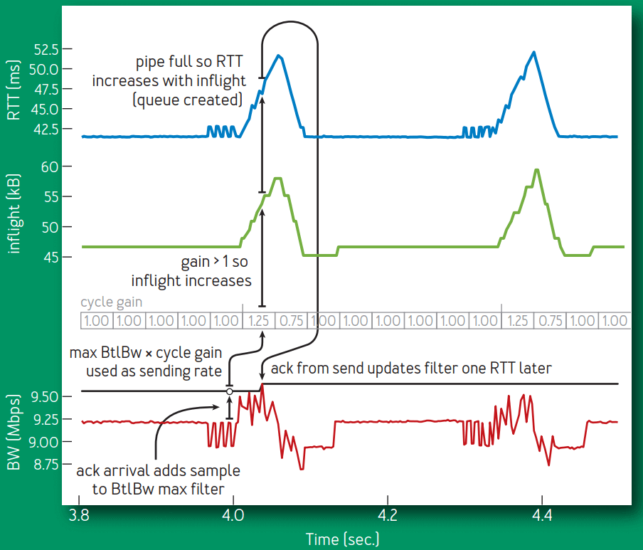
Fig 2. RTT (blue), inflight (green), BtlBw max filter (black) and delivery rate (red) detail
从上到下四条横线:
- RTT
- inflight
-
BtlBw 的估计值(状态)
- 它上面的那行表格是pacing_gain,它是一个固定数组,不断循环;
- 每个时刻使用的 pacing_gain 及其效果在图中是对齐的;
- 每个 gain 会在发送数据时使用,因此是早一个 RTT 窗口;这可以从图中从下往上、再从上往下的整个环路看出来。
- delivery rate(实际传输速率)
几点说明:
- 图中凸起的尖峰是 BBR 使用 pacing_gain 周期切换导致的,目的是判断 BtlBw 是否有增加。
- BBR 在大部分时间都将 inflight 数据量保持在一个 BDP,并用 BtlBw estimate 进行 pace,以此来最小化延迟。 这将瓶颈从链路前移到了发送端,因此发送端是无法看到 BtlBw 升高的。
稳态的收敛过程
BBR 会定期使用 pacing_gain > 1 来均分每个 RTprop interval,增大了发送速率和 inflight 数据量。
下面这是如何保持(或达到新的)稳态的。
考虑链路瓶颈带宽 BtlBw 的两种可能情况:
- 继续保持恒定(大部分情况)
- 突然增大(例如物理链路扩容)
如果 BtlBw 恒定,
- 增加的数据量会在瓶颈处创建一个 queue,这会导致 RTT 变大,但
deliveryRate此时还是恒定的; - 下一个 RTprop 窗口会以
pacing_gain < 1发送数据,从而会将这个 queue 移除。
如果 BtlBw 增大了,
deliveryRate也会增大,那么新的最大值会立即导致 BtlBw 的估计值变大,从而增大了基础 pacing 速率。- 因此,BBR 会以指数级快速收敛到新的瓶颈速率。
图 3 展示了一个原本运行在 10-Mbps/40-ms flow,链路瓶颈突然翻倍到 20 Mbps,平稳运行 20s 之后
又重新回到 10Mbps 的效果:
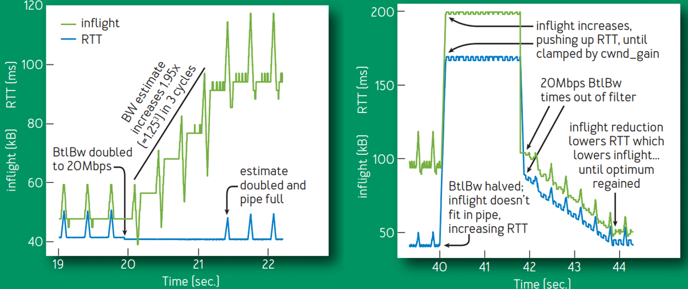
Fig 3. Bandwidth change
BBR 是一个 max-plus 控制系统(一种基于
max()和加法操作的代数)的一个具体使用场景,这是一种基于非标准代数进行控制的新方式12。 这种方式允许 adaptation rate (由 max gain 控制)独立于 queue growth (由 average gain 控制)。 应用到这里,得到的就是一个简单、隐含的控制循环,其中,对物理限制的变化的适应过程, 由代表这些限制的 filters 自动处理。而传统控制系统则需要通过一个复杂状态机连接 起来的多个循环,才能完成同样效果。
4 BBR Flow 行为
4.1 BBR 状态机
现有的实现使用事件相关(event-specific)的算法和代码来处理启动、关闭和丢包恢复等事件。
BBR 使用上一节的两个函数 onAck() 和 send() 处理所有事情,
通过序列化一组“状态”来处理事件,其中“状态”定义为一个 table,其中描述的是一组固定增益和退出条件(fixed gains and exit criteria)。
// include/uapi/linux/inet_diag.h

/* BBR has the following modes for deciding how fast to send: */
enum bbr_mode {
	BBR_STARTUP,	/* ramp up sending rate rapidly to fill pipe */
	BBR_DRAIN,	/* drain any queue created during startup */
	BBR_PROBE_BW,	/* discover, share bw: pace around estimated bw */
	BBR_PROBE_RTT,	/* cut inflight to min to probe min_rtt */
};

/* The pacing_gain values for the PROBE_BW gain cycle, to discover/share bw: */
static const int bbr_pacing_gain[] = {
	BBR_UNIT * 5 / 4,	/* probe for more available bw */
	BBR_UNIT * 3 / 4,	/* drain queue and/or yield bw to other flows */
	BBR_UNIT, BBR_UNIT, BBR_UNIT,	/* cruise at 1.0*bw to utilize pipe, */
	BBR_UNIT, BBR_UNIT, BBR_UNIT	/* without creating excess queue... */
};
状态机:
// net/ipv4/tcp_bbr.c

                                   |
                                   V
                          +---> STARTUP  ----+
                          |        |         |
                          |        V         |
                          |      DRAIN   ----+
                          |        |         |
                          |        V         |
                          +---> PROBE_BW ----+
                          |      ^    |      |
                          |      |    |      |
                          |      +----+      |
                          |                  |
                          +---- PROBE_RTT <--+
-
Startup 状态发生在连接启动时;
- 为了处理跨 12 个量级的互联网链路带宽,Startup 为 BtlBw 实现了一个二分查找,随 着传输速率增加,每次用 2/ln2 增益来 double 发送速率。 这会在 log2BDP 个 RTT 窗口内探测出 BDP,但过程中会导致最多两个 2BDP 的积压(excess queue)。
- 探测出 BtlBw 之后,BBR 转入 Drain 状态。
-
Drain 状态发生在连接启动时;
- Drain 状态利用与 Startup 相反的增益,来排尽那些积压在缓冲区中的数据,
- inflight 数据量降低到一个 BDP 之后,转入 ProbeBW 状态;
-
大部分时间花在 ProbeBW 状态,具体内容就是前面已经介绍的“稳态行为”收敛过程;
4.2 单条 BBR flow 的启动时行为
图 4 展示了一个 10-Mbps/40-ms BBR TCP flow 的前 1 秒,
- 发送端(绿色)和接收端(蓝色)随时间的变化。
- 红色是 CUBIC 发送端在完全相同条件下的行为。
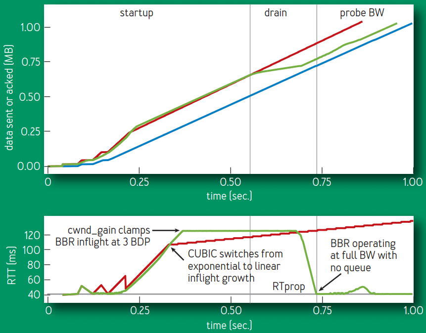
Fig 4. First second of a 10-Mbps, 40-ms BBR flow.
几点解释:
-
上半部分图展示的是 BBR 和 CUBIC 连接的 RTT 随时间的变化。注意,这份数据的时 间参考是 ACK 到达(蓝色),因此,while they appear to be time shifted, events are shown at the point where BBR learns of them and acts.
-
下半部分图中可以看出,BBR 和 CUBIC 的初始行为是类似的,但 BBR 能完全排尽它的 startup queue 而 CUBIC 不能。
CUBIC 算法中没有 inflight 信息,因此它后面的 inflight 还会持续增长(虽然没那么激进),直到 瓶颈 buffer 满了导致丢包,或者接收方的 inflight limit (TCP’s receive window) 达到了。
图 5 是这条 flow 前 8 秒的详情,
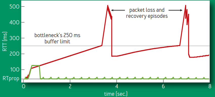
Fig 5. First eight seconds of 10-Mbps, 40-ms CUBIC and BBR flows.
- CUBIC (red) 填满了可用缓冲区,然后每隔几秒就会从 70% to 100%;
- 而 BBR(绿色)启动之后,后面运行时就不会再出现积压。
4.3 共享同一瓶颈的多条 BBR flow 的行为
图 6 展示了共享同一 100-Mbps/10-ms 瓶颈的多条 BBR flow 各自的吞吐,以及如何收敛到公平份额的:
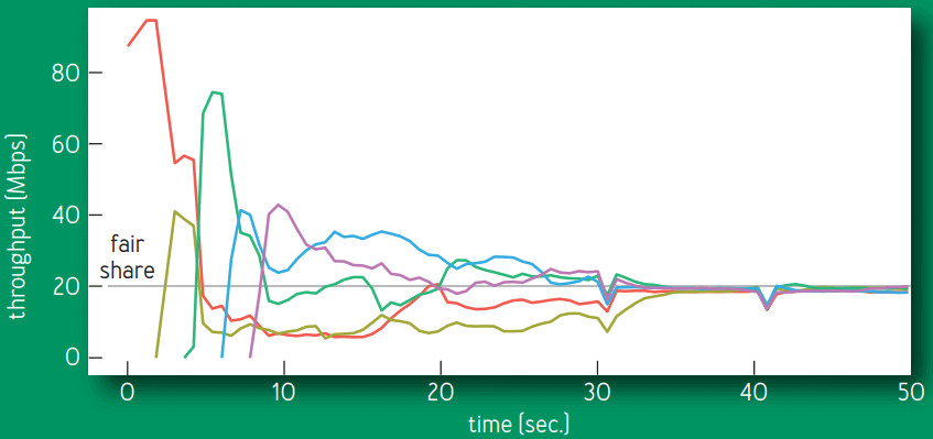
Fig 6. Throughputs of 5 BBR flows sharing a bottleneck
图中向下的几个三角形,是 connection ProbeRTT states,它们的 self-synchronization 加速了最终收敛。
- ProbeBW gain 周期性变化(见前面图 2),使大 flow 将带宽匀给小 flow, 最终每个 flow 都得到一个公平的份额;
- 整个过程非常快(几个 ProbeBW 周期);
但如果某些 flow 已经(短时地)导致积压,后来者会过高估计 RTProp,可能一段时间内 的不公平(收敛时间超出几个 ProbeBW 周期)。
- 要学习到真正的 RTProp,需要通过 ProbeRTT 状态移动到 BDP 的左侧:
- 当 RTProp estimate 持续几秒钟未被更新时(例如,没有测量到一个更低的 RTT) BBR 进入 ProbeRTT,这会将 inflight 降低到每个 RTT 不超过 4 包,然后再返回之前的状态。
大 flow 进入 ProbeRTT 之后会从积压队列中 drain 很多包,因此一些 flows 就能观测 到一个新的 RTprop (new minimum RTT)。这使得它们的 RTprop estimates 在同一时间过 期,因此集中进入 ProbeRTT 状态,这会进一步使积压的数据更快消化,从而使更多 flow 看到新的 RTprop,以此类推。这种分布式协调(distributed coordination)是公平性和稳定性(fairness and stability)的关键。
- BBR 的期望状态是瓶颈队列零积压(an empty bottleneck queue) ,并围绕这个目标不断同步 flow;
- 基于丢包的拥塞控制,期望状态是队列的定期积压和溢出( periodic queue growth and overflow,这会导致延迟放大和丢包),并围绕这个目标不断同步 flow。
5 部署经验
5.1 Google B4 广域网(WAN)部署经验
B4 是 Google 用商用交换机(commodity switches)构建的高速广域网15。
- 这些小缓冲区(shallow-buffered)交换机的丢包主要来自偶发的突发流量;
- 2015 年,Google 开始将 B4 上的生产流量从 CUBIC 切换到 BBR,期间没有出现重大问题;
- 2016 年,所有 B4 TCP 流量都已经切到 BBR。
图 7 可以看出,BBR 的吞吐稳定地比 CUBIC 高 2~25 倍,
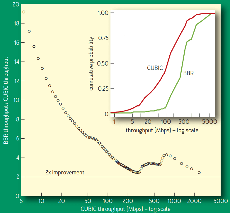
Fig 7. BBR vs. CUBIC relative throughput improvement.
以我们某个活跃的探测器(prober)服务作为实验对象,该服务会创建到远程数据中心的持久 BBR 和 CUBIC 连接,
然后每分钟传输 8MB 数据。探测器之间会通过北美、欧洲和亚洲的多条跨洲或洲内 B4 路径通信。
但按照我们的理论估计,BBR 的性能应该比这个更好,
- 排查之后发现,75% 的 BBR 连接都受限于内核 TCP 的接收缓冲区,我们的网络运营团 队之前有意将这个参数调低了(设置为 8MB),目的是防止 CUBIC MB 量级的积压数据 泛洪(跨洲 8-MB/200-ms RTT 将导致最大 335-Mbps 带宽占用),
- 手动将 US-Europe 的一条路径上的接收缓冲区调大之后,BBR 立即达到了 2Gbps 的带宽 —— 而 CUBIC 仍然只能到达 15Mbps —— 133 倍的提升,正如 Mathis 等人的预测17。
这巨大的提升是 BBR 没有将丢包作为拥塞指示器(not using loss as a congestion indicator)的一个直接结果。 为达到全速带宽,现有的基于丢包的拥塞控制,要求丢包率低于 BDP 的 inverse square 17 (e.g., 小于 one loss per 30 million packets for a 10-Gbps/100-ms path)
Figure 8 比较了不同丢包率下的实际吞吐量:
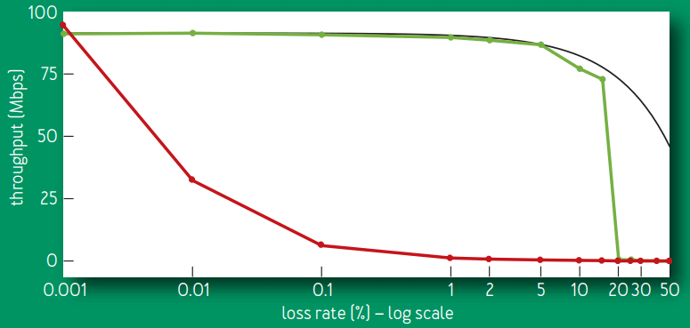
Fig 8. BBR vs. CUBIC goodput for 60-second flows on a 100-Mbps/100-ms link with 0.001 to 50 percent random loss.
最大可能的吞吐是 链路速率乘以 * (1 - lossRate),
- CUBIC 的吞吐在丢包率
0.1%时下降到了原来的 1/10 倍,在丢包率 1% 时完全跌零了。 - BBR 的吞吐 在丢包率小于 5% 时能维持在最大值,在丢包率超过
15%之后才开始急剧下降。
CUBIC 的 loss tolerance 是其算法的一个结构特性(structural property), 而 BBR 中它是一个配置参数。当 BBR 的丢包率接近 ProbeBW 峰值增益时, 测量真实 BtlBw 的传输速率的概率将剧烈下降,导致最大值过滤器(the max filter)将 产生过低估计(underestimate)。
5.2 YouTube 边缘网络部署经验
BBR 已经部署到了 Google.com 和 YouTube 视频服务器上。我们在小规模灰度,一小部分用户会随机被分到 BBR 或 CUBIC。
- 以 YouTube 的所有体验质量指标来衡量,BBR 给用户带来的提升都非常明显,这可能是 由于 BBR 的行为更加一致和可预测(consistent and predictable)。
- BBR 只是略微提升了 Youtube 的连接吞吐(connection throughput),这是因为 YouTube 已经将服务器的 streaming rate 充分控制在 BtlBw 以下,以最小化缓冲区膨胀(bufferbloat)和多次缓冲(rebuffer)问题。
- 但即使是在这样的条件下,BBR 仍然将全球范围内 RTT 的中值平均降低了 53%, 而在发展中国家,这个降低的百分比更是达到了 80%。
图 9 展示了 BBR vs. CUBIC 的中值 RTT 提升,数据来自一个星期内从五个大洲采集的超 过 2 亿条 YouTube playback 连接,
- 在全球 70 亿移动互联用户中,超过一半是通过
8-114kbps的 2.5G 网络接入的5, 这会导致很多已知问题,问题的根源在于,基于丢包的拥塞控制有所谓的缓冲区填充倾向 (buffer-filling propensities)3; - 这些系统的瓶颈链路通常位于在 SGSN (serving GPRS support node)18 和移动设备之间。 SGSN 软件运行在有足够内存的标准 PC 平台上,因此在互联网和移动设备之间经常有数 MB 的缓冲区。
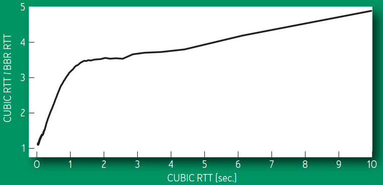
Fig 9. BBR vs. CUBIC median RTT improvement.
图 10 比较(仿真)了 BBR 和 CUBIC 的 SGSN Internet-to-mobile delay。
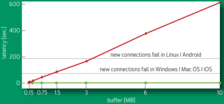
Fig 10. Steady-state median RTT variation with link buffer size.
稳态时的 RTT 随链路缓冲区大小的变化,链路物理特性:128-Kbps/40-ms,8 BBR (green) / CUBIC (red) flows。
不管瓶颈缓冲区大小和活跃的 flow 数量如何,BBR 几乎一直将队列(延迟)保持在最小;
CUBIC flow 永远会填满缓冲区, 因此延迟随着 buffer size 线性增长。
几条水平线处表示的含义非常重要:
- 除了连接建连时的 SYN 包之外, TCP 已经适应到了一个非常大的 RTT 延迟(初始 SYN 包延迟由操作系统 hardcode,因此不会很大)。
- 当移动设备通过一个大缓冲区的 SGSN 接收大块数据时(例如,手机软件自动更新), 那这个设备就无法连接到互联网上的任何东西,直到队列被清空(SYN-ACK accept packet 被延迟的时间大于固定 SYN timeout)。
Linux 的初始超时时间是 1s,见 Customize TCP initial RTO (retransmission timeout) with BPF。 译注。
6 问题讨论
6.1 移动蜂窝网络中的自适应带宽
蜂窝网络会根据每个用户的数据包排队(queue of packets)情况来调整每个用户的带宽 (adapt per-subscriber bandwidth)。
早期版本的 BBR 通过针对性调优来产生非常小的队列,导致在低速情况下连接会卡住(stuck at low rates)。
增大峰值 ProbeBW pacing_gain 来产生更大的队列,会使得卡住的情况大大减少,这暗示
大队列(缓冲区)对某些网络也不是坏事。
使用当前的 1.25 × BtlBwpeak gain,BBR 在任何网络上都不会比 CUBIC 差。
6.2 延迟和聚合应答
蜂窝、WIFI 和有线宽带网络经常会延迟和聚合 ACK(delay and aggregate) 1。当 inflight 限制到单个 BDP 时,这会导致因为数据太少而导致的卡顿( throughput-reducing stalls)。
将增大 ProbeBW cwnd_gain 增大到 2 使得 BBR 能在估计的传输速率上持续平稳发送,即使 ACK 被延迟了一个 RTT,这显著避免了卡顿(stalls)。
6.3 入向流量整形(Token-Bucket Policers)
BBR 在 YouTube 部署之后,我们发现世界上大部分 ISP 都会用 TBP 来对接收到的流量进行处理(mangle) 7。
- 连接刚启动时,bucket 通常是满的,因此 BBR 能学到底层网络的 BtlBw,
- 一旦 bucket 空了,所有发送速率快于(比 BtlBw 低一些的)bucket 填充速率的包,都会被丢弃,
- BBR 最终会学到这个新的传输速率,但 ProbeBW gain cycle 会导致持续的、少量的丢包(continuous moderate losses)。
为最小化上游带宽浪费,以及最小化因为丢包而导致的应用延迟增加,我们给 BBR 添加了 policer detection 和一个显式 policer 模型,并还在持续研究更好的方式来减缓 policer 带来的损失。
更多入向流量整形(policing)内容,可参考: (译)《Linux 高级路由与流量控制手册(2012)》第九章:用 tc qdisc 管理 Linux 网络带宽。 译注。
6.4 与基于丢包的拥塞控制的竞争
不管是与其他 BBR flow 竞争,还是与基于丢包的拥塞控制竞争, BBR 都能收敛到瓶颈带宽的一个公平份额。
即使基于丢包的拥塞控制填满了可用缓冲区,ProbeBW 仍然能健壮地将 BtlBw estimate 朝着 flow 的公平份额移动,ProbeRTT 也是类似。
但是,不受通信双方控制的路由器缓冲区会比 BDP 大好几倍,导致 long-lived loss-based competitors 占用大量队列,因此获得超出其公平的份额。 如何解决(缓解)这个问题也是目前业内很热门的一个研究方向。
7 总结
重新思考拥塞控制让我们发掘出了这个古老世界的许多新东西。 相比于使用丢包、缓冲区大小等等这些与拥塞只是弱相关的事件, BBR 以 Kleinrock 关于拥塞的规范化模型和与之相关的最佳工作位置作为出发点。
关键的两个参数 —— 延迟和带宽 —— 无法同时确定, 这一结论看似绝望,但我们发现通过对二者进行顺序估计(estimated sequentially)能绕开这一限制。具体来说,我们使用控制与估计理论领域的一些最新进 展,创建了一个简单的分布式控制循环,后者能接近最优值,在充分利用网络的 同时还能保持一个很小的缓冲队列。
Google BBR 的实现已经合并到 Linux 内核,关于一些实现细节见本文附录。
BBR is deployed on Google’s B4 backbone, improving throughput by orders of magnitude compared with CUBIC. It is also being deployed on Google and YouTube Web servers, substantially reducing latency on all five continents tested to date, most dramatically in developing regions.
BBR 只运行在发送端,无需协议、接收端或网络的改动,因此可以做到 灰度(增量)部署。它只依赖 RTT 和应答包,因此大部分互联网传输协议都能实现这个算法。
The authors are members of Google’s make-tcp-fast project, whose goal is to evolve Internet transport via fundamental research and open source software. Project contributions include TFO (TCP Fast Open), TLP (Tail Loss Probe), RACK loss recovery, fq/pacing, and a large fraction of the git commits to the Linux kernel TCP code for the past five years.
The authors can be contacted at bbr-dev@googlegroups.com.
致谢
- The authors are grateful to Len Kleinrock for pointing out the right way to do congestion control.
- We are indebted to Larry Brakmo for pioneering work on Vegas2 and New Vegas congestion control that presaged many elements of BBR, and for advice and guidance during BBR’s early development.
- We would also like to thank Eric Dumazet, Nandita Dukkipati, Jana Iyengar, Ian Swett, M. Fitz Nowlan, David Wetherall, Leonidas Kontothanassis, Amin Vahdat, and the Google BwE and YouTube infrastructure teams for their invaluable help and support.
附录:详细描述
顺序探测状态机(A State Machine for Sequential Probing)
The pacing_gain controls how fast packets are sent relative to BtlBw and is key
to BBR’s ability to learn. A pacing_gain > 1 increases inflight and decreases
packet inter-arrival time, moving the connection to the right on figure 1. A
pacing_gain < 1 has the opposite effect, moving the connection to the left.
BBR uses this pacing_gain to implement a simple sequential probing state machine that alternates between testing for higher bandwidths and then testing for lower round-trip times. (It’s not necessary to probe for less bandwidth since that is handled automatically by the BtlBw max filter: new measurements reflect the drop, so BtlBw will correct itself as soon as the last old measurement times out of the filter. The RTprop min filter automatically handles path length increases similarly.)
If the bottleneck bandwidth increases, BBR must send faster to discover this. Likewise, if the actual round-trip propagation delay changes, this changes the BDP, and thus BBR must send slower to get inflight below BDP in order to measure the new RTprop. Thus, the only way to discover these changes is to run experiments, sending faster to check for BtlBw increases or sending slower to check for RTprop decreases. The frequency, magnitude, duration, and structure of these experiments differ depending on what’s already known (startup or steady-state) and sending app behavior (intermittent or continuous).
稳态行为(Steady-State Behavior)
BBR flows spend the vast majority of their time in ProbeBW state, probing for bandwidth using an approach called gain cycling, which helps BBR flows reach high throughput, low queuing delay, and convergence to a fair share of bandwidth. With gain cycling, BBR cycles through a sequence of values for the pacing_gain. It uses an eight-phase cycle with the following pacing_gain values: 5/4, 3/4, 1, 1, 1, 1, 1, 1. Each phase normally lasts for the estimated RTprop. This design allows the gain cycle first to probe for more bandwidth with a pacing_gain above 1.0, then drain any resulting queue with a pacing_gain an equal distance below 1.0, and then cruise with a short queue using a pacing_gain of 1.0. The average gain across all phases is 1.0 because ProbeBW aims for its average pacing rate to equal the available bandwidth and thus maintain high utilization, while maintaining a small, well-bounded queue. Note that while gain cycling varies the pacing_gain value, the cwnd_gain stays constant at two, since delayed and stretched acks can strike at any time (see the section on Delayed and Stretched Acks).
Furthermore, to improve mixing and fairness, and to reduce queues when multiple BBR flows share a bottleneck, BBR randomizes the phases of ProbeBW gain cycling by randomly picking an initial phase—from among all but the 3/4 phase—when entering ProbeBW. Why not start cycling with 3/4? The main advantage of the 3/4 pacing_gain is to drain any queue that can be created by running a 5/4 pacing_gain when the pipe is already full. When exiting Drain or ProbeRTT and entering ProbeBW, there is no queue to drain, so the 3/4 gain does not provide that advantage. Using 3/4 in those contexts only has a cost: a link utilization for that round of 3/4 instead of 1. Since starting with 3/4 would have a cost but no benefit, and since entering ProbeBW happens at the start of any connection long enough to have a Drain, BBR uses this small optimization.
BBR flows cooperate to periodically drain the bottleneck queue using a state called ProbeRTT. In any state other than ProbeRTT itself, if the RTProp estimate has not been updated (i.e., by getting a lower RTT measurement) for more than 10 seconds, then BBR enters ProbeRTT and reduces the cwnd to a very small value (four packets). After maintaining this minimum number of packets in flight for at least 200 ms and one round trip, BBR leaves ProbeRTT and transitions to either Startup or ProbeBW, depending on whether it estimates the pipe was filled already.
BBR was designed to spend the vast majority of its time (about 98 percent) in ProbeBW and the rest in ProbeRTT, based on a set of tradeoffs. ProbeRTT lasts long enough (at least 200 ms) to allow flows with different RTTs to have overlapping ProbeRTT states, while still being short enough to bound the performance penalty of ProbeRTT’s cwnd capping to roughly 2 percent (200 ms/10 seconds). The RTprop filter window (10 seconds) is short enough to allow quick convergence if traffic levels or routes change, but long enough so that interactive applications (e.g., Web pages, remote procedure calls, video chunks) often have natural silences or low-rate periods within the window where the flow’s rate is low enough or long enough to drain its queue in the bottleneck. Then the RTprop filter opportunistically picks up these RTprop measurements, and RTProp refreshes without requiring ProbeRTT. This way, flows typically need only pay the 2 percent penalty if there are multiple bulk flows busy sending over the entire RTProp window.
启动行为(Startup Behavior)
When a BBR flow starts up, it performs its first (and most rapid) sequential probe/drain process. Network-link bandwidths span a range of 1012— from a few bits to 100 gigabits per second. To learn BtlBw, given this huge range to explore, BBR does a binary search of the rate space. This finds BtlBw very quickly (log2BDP round trips) but at the expense of creating a 2BDP queue on the final step of the search. BBR’s Startup state does this search and then the Drain state drains the resulting queue.
First, Startup grows the sending rate exponentially, doubling it each round. To achieve this rapid probing in the smoothest possible fashion, in Startup the pacing_gain and cwnd_gain are set to 2/ln2, the minimum value that will allow the sending rate to double each round. Once the pipe is full, the cwnd_gain bounds the queue to (cwnd_gain - 1) × BDP.
During Startup, BBR estimates whether the pipe is full by looking for a plateau in the BtlBw estimate. If it notices that there are several (three) rounds where attempts to double the delivery rate actually result in little increase (less than 25 percent), then it estimates that it has reached BtlBw and exits Startup and enters Drain. BBR waits three rounds in order to have solid evidence that the sender is not detecting a delivery-rate plateau that was temporarily imposed by the receive window. Allowing three rounds provides time for the receiver’s receive-window autotuning to open up the receive window and for the BBR sender to realize that BtlBw should be higher: in the first round the receive-window autotuning algorithm grows the receive window; in the second round the sender fills the higher receive window; in the third round the sender gets higher delivery-rate samples. This three-round threshold was validated by YouTube experimental data.
In Drain, BBR aims to quickly drain any queue created in Startup by switching to a pacing_gain that is the inverse of the value used during Startup, which drains the queue in one round. When the number of packets in flight matches the estimated BDP, meaning BBR estimates that the queue has been fully drained but the pipe is still full, then BBR leaves Drain and enters ProbeBW.
Note that BBR’s Startup and CUBIC’s slow start both explore the bottleneck capacity exponentially, doubling their sending rate each round; they differ in major ways, however. First, BBR is more robust in discovering available bandwidth, since it does not exit the search upon packet loss or (as in CUBIC’s Hystart10) delay increases. Second, BBR smoothly accelerates its sending rate, while within every round CUBIC (even with pacing) sends a burst of packets and then imposes a gap of silence. Figure 4 demonstrates the number of packets in flight and the RTT observed on each acknowledgment for BBR and CUBIC.
应对突发流量(Reacting to Transients)
The network path and traffic traveling over it can make sudden dramatic changes. To adapt to these smoothly and robustly, and reduce packet losses in such cases, BBR uses a number of strategies to implement the core model. First, BBR treats cwnd_gain×BDP as a target that the current cwnd approaches cautiously from below, increasing cwnd by no more than the amount of data acknowledged at any time. Second, upon a retransmission timeout, meaning the sender thinks all in-flight packets are lost, BBR conservatively reduces cwnd to one packet and sends a single packet (just like loss-based congestion-control algorithms such as CUBIC). Finally, when the sender detects packet loss but there are still packets in flight, on the first round of the loss-repair process BBR temporarily reduces the sending rate to match the current delivery rate; on second and later rounds of loss repair it ensures the sending rate never exceeds twice the current delivery rate. This significantly reduces transient losses when BBR encounters policers or competes with other flows on a BDP-scale buffer.
References
- Abrahamsson, M. 2015. TCP ACK suppression. IETF AQM mailing list; https://www.ietf.org/mail-archive/web/aqm/current/msg01480.html.
- Brakmo, L. S., Peterson, L.L. 1995. TCP Vegas: end-to-end congestion avoidance on a global Internet. IEEE Journal on Selected Areas in Communications 13(8): 1465-1480.
- Chakravorty, R., Cartwright, J., Pratt, I. 2002. Practical experience with TCP over GPRS. In IEEE GLOBECOM.
- Corbet, J. 2013. TSO sizing and the FQ scheduler. LWN.net; https://lwn.net/Articles/564978/.
- Ericsson. 2015 Ericsson Mobility Report (June); https://www.ericsson.com/res/docs/2015/ericsson-mobility-report-june-2015.pdf.
- ESnet. Application tuning to optimize international astronomy workflow from NERSC to LFI-DPC at INAF-OATs; http://fasterdata.es.net/data-transfer-tools/case-studies/nersc-astronomy/.
- Flach, T., Papageorge, P., Terzis, A., Pedrosa, L., Cheng, Y., Karim, T., Katz-Bassett, E., Govindan, R. 2016. An Internet-wide analysis of traffic policing. In ACM SIGCOMM: 468-482.
- Gail, R., Kleinrock, L. 1981. An invariant property of computer network power. In Conference Record, International Conference on Communications: 63.1.1-63.1.5.
- Gettys, J., Nichols, K. 2011. Bufferbloat: dark buffers in the Internet. acmqueue 9(11); http://queue.acm.org/detail.cfm?id=2071893.
- Ha, S., Rhee, I. 2011. Taming the elephants: new TCP slow start. Computer Networks 55(9): 2092-2110.
- Ha, S., Rhee, I., Xu, L. 2008. CUBIC: a new TCP-friendly high-speed TCP variant. ACM SIGOPS Operating Systems Review 42(5): 64-74.
- Heidergott, B., Olsder, G. J., Van Der Woude, J. 2014. Max Plus at Work: Modeling and Analysis of Synchronized Systems: a Course on Max-Plus Algebra and its Applications. Princeton University Press.
- Jacobson, V. 1988. Congestion avoidance and control. ACM SIGCOMM Computer Communication Review 18(4): 314-329.
- Jaffe, J. 1981. Flow control power is nondecentralizable. IEEE Transactions on Communications 29(9): 1301-1306.
- Jain, S., Kumar, A., Mandal, S., Ong, J., Poutievski, L., Singh, A., Venkata, S., Wanderer, J., Zhou, J., Zhu, M., et al. 2013. B4: experience with a globally-deployed software defined WAN. ACM SIGCOMM Computer Communication Review 43(4): 3-14.
- Kleinrock, L. 1979. Power and deterministic rules of thumb for probabilistic problems in computer communications. In Conference Record, International Conference on Communications: 43.1.1-43.1.10.
- Mathis, M., Semke, J., Mahdavi, J., Ott, T. 1997. The macroscopic behavior of the TCP congestion avoidance algorithm. ACM SIGCOMM Computer Communication Review 27(3): 67-82.
- Wikipedia. GPRS core network serving GPRS support node.